In this project, I implemented a path tracer, which renders three-dimensional scenes by integrating over the illuminance arriving at a single point on an object. I first implemented an algorithm that traces a ray over a pixel when taking a certain amount of samples-per-pixel. Calculating barycentric coordinates, I applied triangle-ray intersection detection as well as sphere intersection with the quadratic formula. Since testing for detection with every primitive in a scene can be costly, I implemented a Bounding Volume Hierarchy tree structure to test for intersection of larger volumes before checking individual primitives. This sped up the process of rendering immensely. Next, I applied a direct illumination which accounts for illumination on objects in a scene that comes straight from light sources. I did this in two ways: by sampling uniformly in a hemisphere and by sampling each light directly (areas in the hemisphere with greater importance). While this only accounts for the light coming straight from the source, Global Illumination accounts for more bounces, which I applied next using a recursive algorithm and a termination factor. I finally calculated adaptive sampling, which alters the amount of samples per pixel based on how long it takes the pixel to converge.
Part 1: Ray Generation and Scene Intersection
First, I implemented ray generation by averaging a spectrum of the irradiance over single pixels, taking ns_aa samples per pixel. After calculating random sample points and adding them to the (x, y) pixel coordinates, I scaled down the coordinates by sampleBuffer.w and sampleBuffer.h and passed them to the camera. Next, to generate the camera ray, I converted the input point to a point on the sensor with linear interpolation over the bottom left and top right corners of the sensor plane defined by:
Vector3D(-tan(radians(hFov)*.5), -tan(radians(vFov)*.5),-1) &
Vector3D( tan(radians(hFov)*.5),  tan(radians(vFov)*.5),-1)
I converted the ray’s direction to world space with the c2w matrix and moved on to triangle intersection. It was extremely important to note that the ray’s t values gave a range of intersection times, which needed to be compared to the triangle’s t value. The ray’s max_t value could then be updated if there was an intersection to short-circuit checks to farther away primitives. Using the Moller Trumbore algorithm, I found the triangle’s barycentric coordinates. Once an intersection was found, I filed the intersection structure with the bsdf, primitive, the ray’s t value, and the surface normal of the hit point calculated using the barycentric coordinates. The biggest issue I ran into at this stage was forgetting to normalize the direction of the ray after the world coordinate transform. Once normalized, I was able to test a render with normal shading.
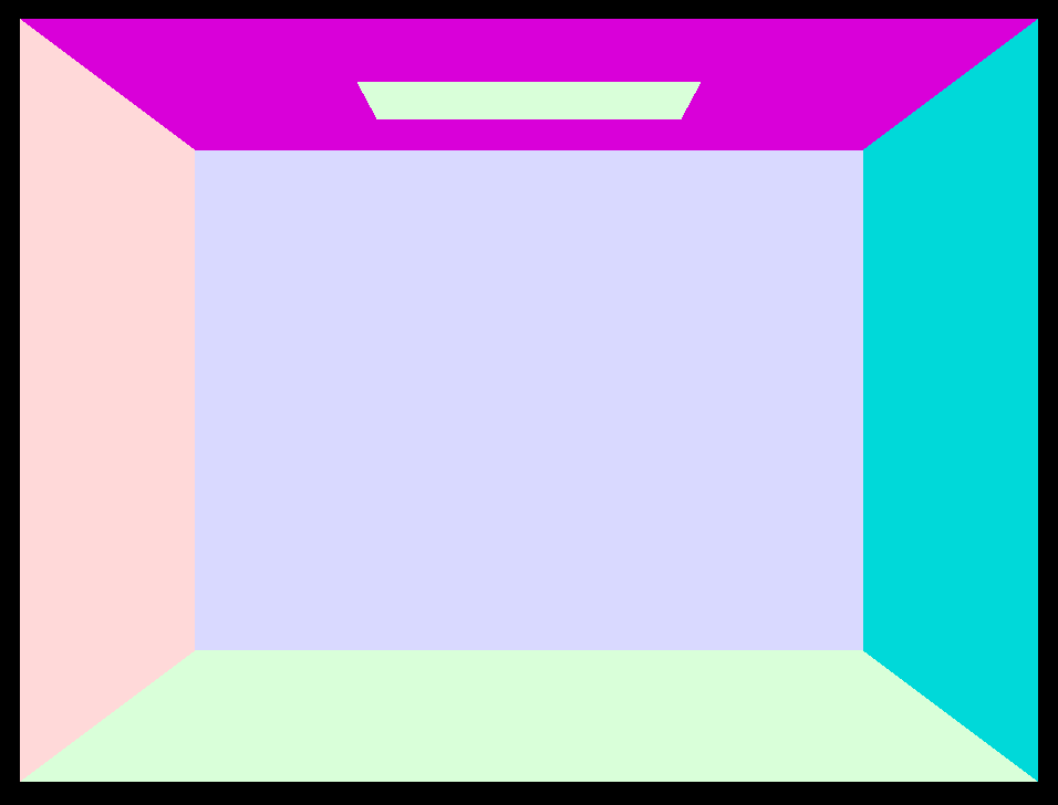 CBspheres_lambertian.dae after generating camera rays and triangle intersection
|
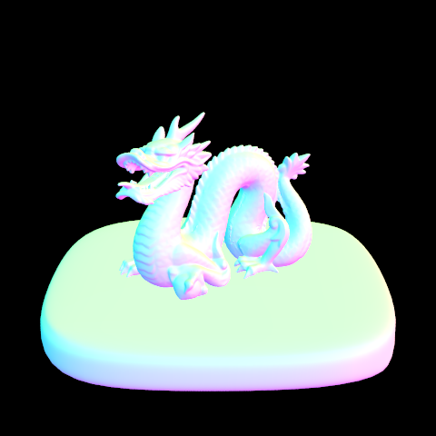
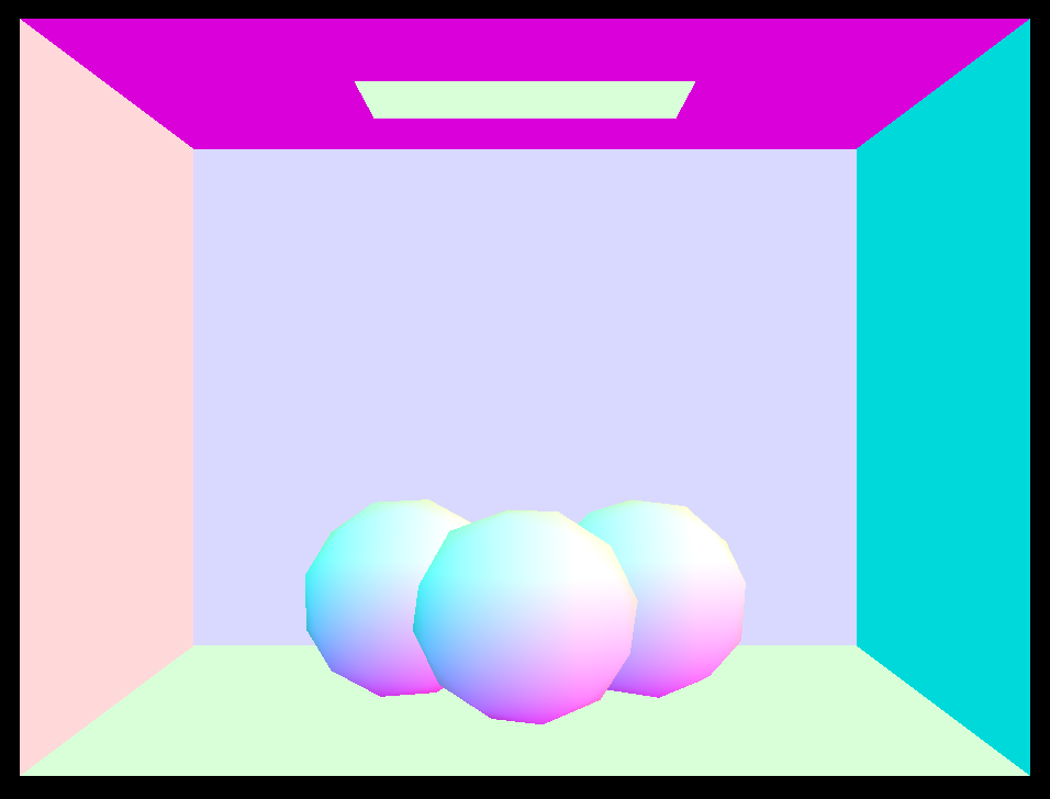
Next I implemented sphere intersection, which was similar to triangle intersection. I used the quadratic formula to determine the number of intersections and their locations. I checked the min_t and max_ t in the same way as with triangle intersection. While filling in the intersection structure, I had trouble computing the normal vecotor, and later figured out that I could pass the ray’s origin + direction * max_t value (ray equation) into the normal function in order to get the vector. Below is the result of the sphere intersection as well as some other .dae files.
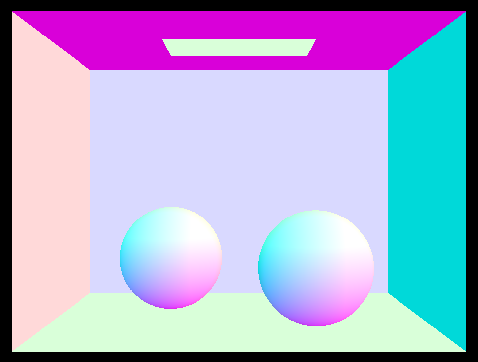 CBspheres_lambertian.dae
|
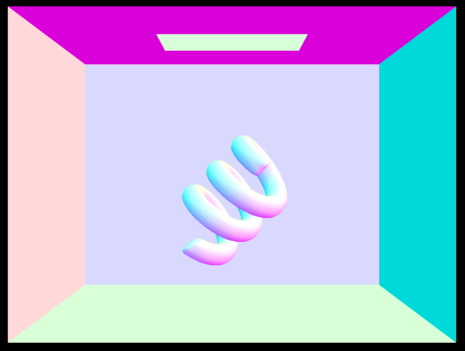 CBcoil.dae
|
 CBgems.dae
|
Part 2: Bounding Volume Hierarchy
To accelerate render time, especially for scenes with many primitives, I implemented a Bounding Volume Hierarchy(bvh). A BVH is a binary tree structure containing primitives in a scene that get placed in left or right nodes depending on where the objects center is relative to a chosen hit point. First, I built the hierarchy with a node structure containing left and right members. I checked to see if the number of primitives in the scene was less than the max leaf size, and if so the BVH construction was complete. If not, I took the largest axis of the bounding box’s extent of the scene and decided on a split point by averaging out the centroids of the primitives. If a primitive’s centroid on the chosen axis was less than the split point on the same axis, I put it in the left child vector and if it is greater I put it in the right child vector. In the case that all of the children are on one side of the split point, I used the midpoint of the primitives' centers as the heuristic, which ensured no empty child nodes.
To check for intersection while traversing the BVH, we check for intersection with each node’s bounding box. I calculated six values (one for each face of the box) using the min and max coordinates on each axis and the plane intersection equation:
t = (p’ – o) /d
I performed a check for the computed min/max values on each axis to make sure that the min was less than the max, and if not, to switch them since that meant the ray was hitting that plane from the opposite direction. I then took the min of the max values and the max of the min values and determined that an intersection occurred within these new bounds (t_min, t_max). We take the min of the maxs and the max of of the mins because we want to constrain our bounds to the box itself, instead of having t values that still lie on the plane but in a position far away from the box. Once detection of an intersection was complete, I continued with traversing the hierarchy. If the current node was a leaf, I looped through it to check for primitive intersections. If not, I recursed on the left and right children returning if there was an intersection in either call. If there was an intersection, we did not have to worry about intersection data since the intersect call to the primitive took care of filling in the intersect struct for us. Below are renders of scenes that became renderable with the BVH implementation.
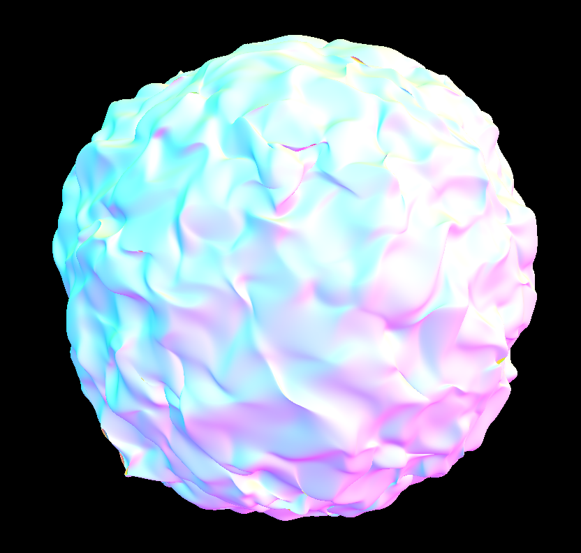 CBblob.dae
|
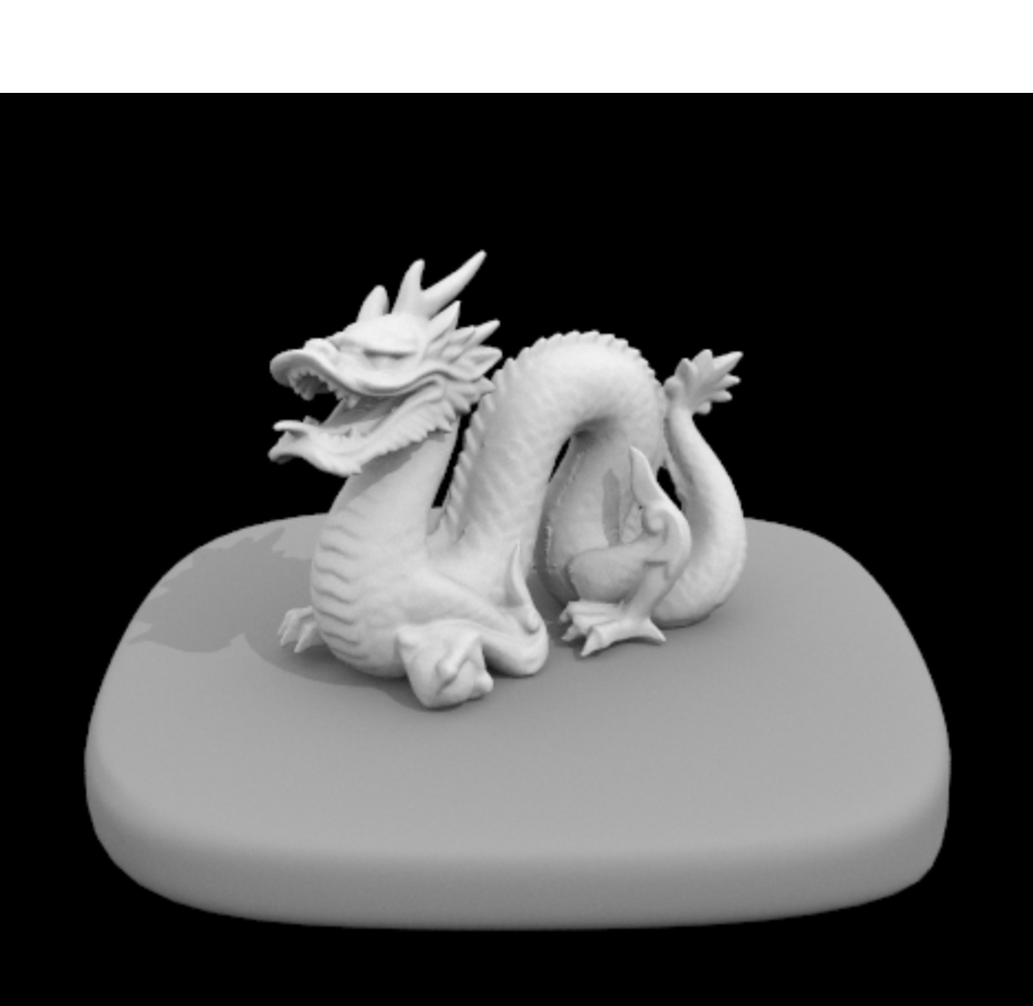
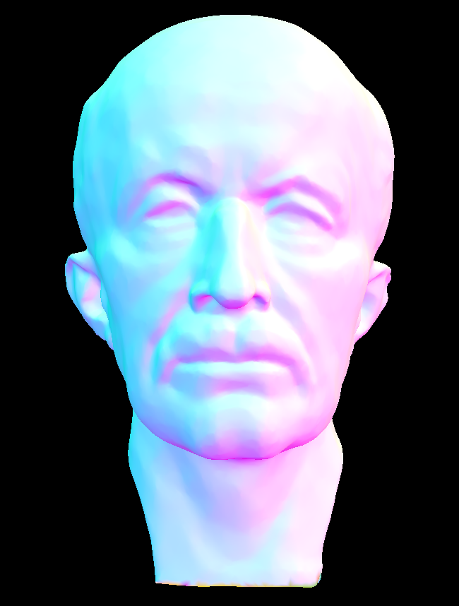 maxplanck.dae
|
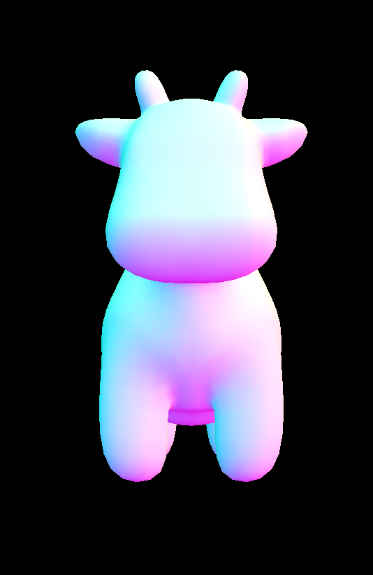 cow.dae
|
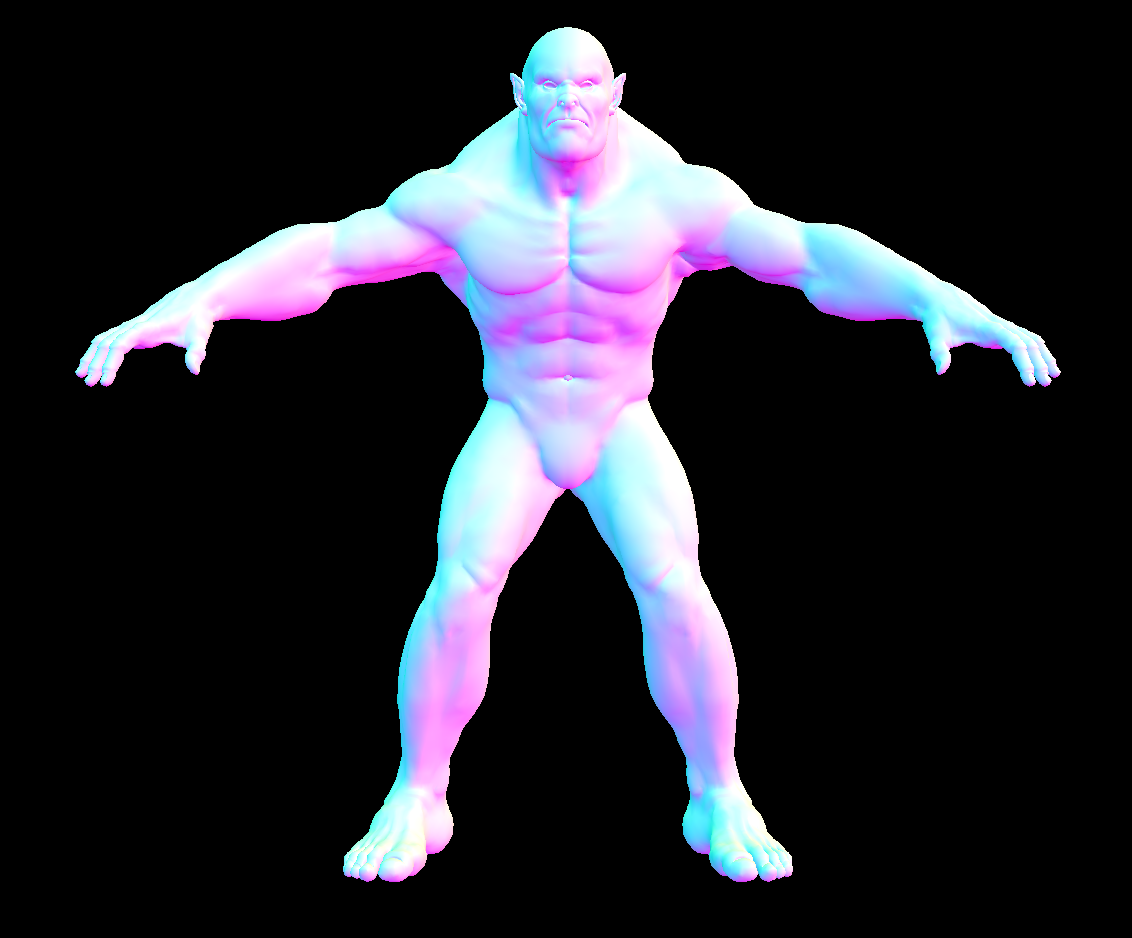 beast.dae
|
This method accelerated intersection in a large way. The render time for the cow before the BVH implementation took 3-4 minutes, but took about 3 seconds after the implementation. Since we are now rejecting nodes with bounding boxes that never are intersected, we no longer have to loop through entire groups primitives and test for an intersection that will never occur. This cuts down runtime from linear to log (if we have a good heuristic), thus saving us some computational energy.
Part 3: Direct Illumination
For the next part, I calculated direct lighting, which acounts for illuminated parts of a scene that have taken paths directly from a light source. I first implemented hemisphere sampling, which samples uniformly in a hemisphere around the scene. Looping through the number of samples for the area light, I calculated the sample and converted it to world coordinates. I cast a shadow ray from the hit point scaled by the sample * EPS_D value in the direction of the world coordinate sample. I tested for an intersection with the ray and a new intersection structure, and if it intersected I calculated the emission, scaling it by the cosine term and the BSDF. Finally, I averaged by the number of samples and added the spectrum to the total emission.
Next, I implemented importance sampling which samples each light directly versus sampling uniformly in a hemisphere, ultimately reducing noise in renders. Looping through the lights, I determined if each light was a delta light. If so, we only have to take one sample, since they will always fall in the same place. If not, I continued and looped through the total amount of samples. I called Sample_L, which returns the direction from the hit point to the light source and a PDF for that direction by pointer. I cast a shadow ray from the hit point to determine if it hit other objects before it reached the sampled light position. If it did not hit any objects, we know that it gets to the light and we can add the spectrum to the total emission, scaled by a cosine term and the BSDF.
Below are the results of rendering with 1 sample per pixel and with increasingly more light rays(1, 4, 16, 16). Noise levels in soft shadows were quite large until 16 light rays where softer transitions at shadow edges began to appear. We can more accurately estimate the radiance of each pixel by averaging out the spectrum in a scene with more light rays, exemplified in these renders.
 1 sample, 1 light ray
|
 1 sample, 4 light rays
|
 1 sample, 16 light rays
|
 1 sample, 64 light rays
|
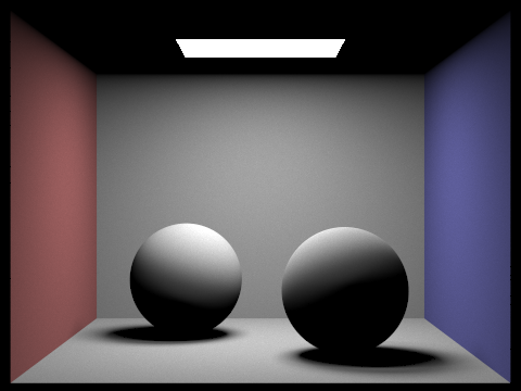
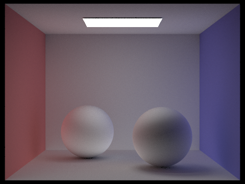
Results from uniform hemisphere sampling versus importance sampling with the same command line arguments come out quite different. While soft shadows are present in both renders, there is much more noise in the hemisphere sampling. Since hemisphere sampling produces rays at the horizon (which end up having very little effect on the render), we can ensure that rays are cast above the horizon towards light sources with importance sampling, giving priority to rays that contribute more to the result than others. Thus, the final render is less noisy with importance sampling, while hemisphere sampling gives equal priority to rays uniformly.
 64 samples, 32 light rays, hemisphere
|
 64 samples, 32 light rays, importance
|
Part 4: Global Illumination
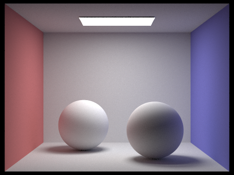 CBspheres.dae, 1024 samples
|
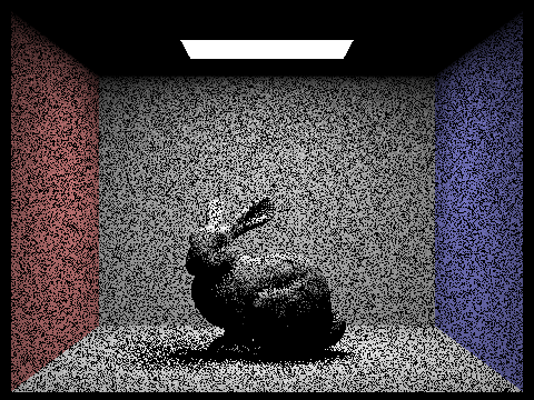
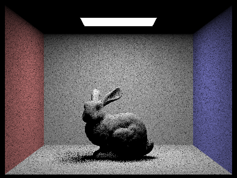
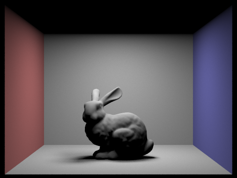
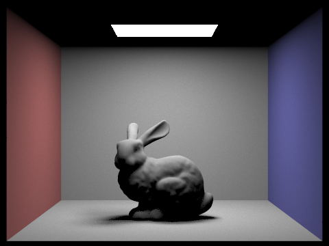
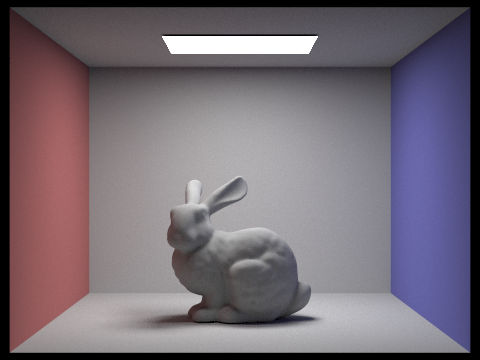
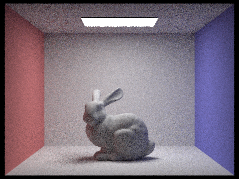
 CBbunny.dae, 1024 samples
|
Both hemisphere and importance sampling only account for illumination that has taken a path directly from a light source, but Global Illumination adds up a series of light bounces depending on the max ray depth argument. Overall, Global Illumination takes into account light reflected from other surfaces in the scene. To do this we trace rays recursively until they hit a light source. Some rays may bounce infinitely, so we use Russian Roulette to decide when to randomly terminate rays. First, I set the final spectrum to be one bounce radiance, which is either hemisphere or importance sampling. I used the coin_flip function with a 0.7 probability for termination. I decrement the ray’s depth by 1 each bounce, as well. If the max ray depth is greater than 1 we know we always trace at least one indirect bounce. I checked for this and tested if there was an intersection before deciding whether to terminate or keep recursing. I finally convert this incoming radiance to outgoing radiance with a cosine scaling factor, the BSDF, the pdf, and 1-termination probability. I add this recursive call the the overall result.
Below are comparisions of only direct illuminationa and only indirect. To achieve indirect illuminaton, we must subtract the call to one bounce from our result, so we only add up the subsequent recursive calls/bounces of light.
 1024 samples per pixel, direct
|
 1024 samples per pixel, indirect
|
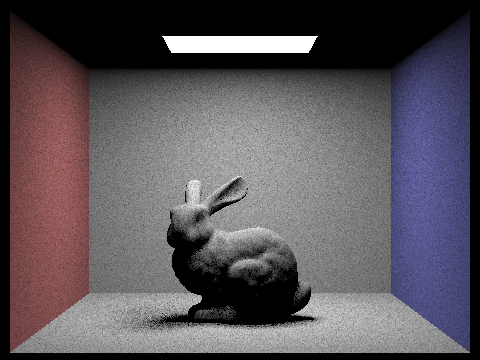
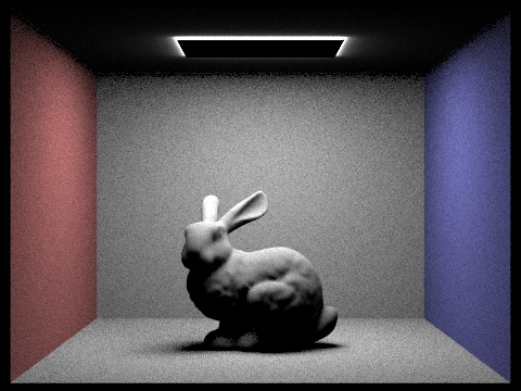
Next, I compared renders with different max ray depths. As expected, with a max ray depth of 1, we get direct illumination. We only see the effects of global illumination with a max ray depth greater than 1.
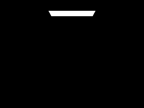 max ray depth 0
|
 max ray depth 1
|
 max ray depth 2
|
 max ray depth 3
|
 max ray depth 100
|
Using 4 light rays, I compared the renders of various samples per pixel rates.
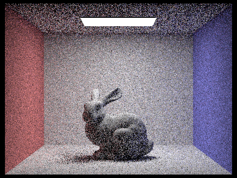 1 sample
|
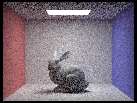 2 samples
|
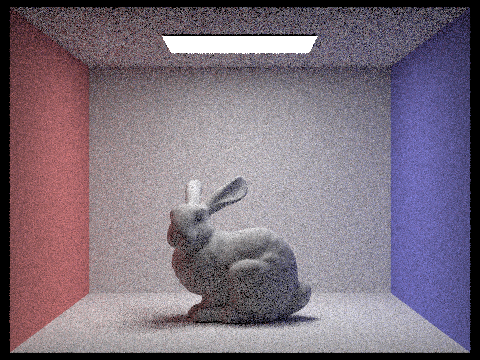 4 samples
|
 8 samples
|
 16 samples
|
 64 samples
|
|
1024 samples
|
Part 5: Adaptive Sampling
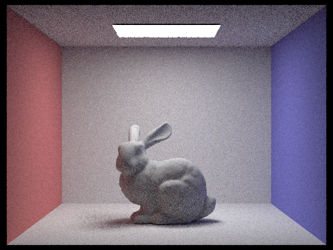
 2048 samples
|
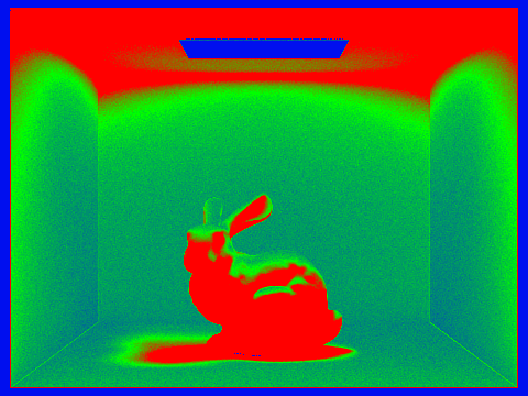 sample rate result
|
For the final part of the project, I implemented adaptive sampling, which changes the sample rate based on how quickly a pixel converges. While some pixels require more samples to get rid of noise, others converge fast. Thus, we can concentrate higher sample rates in certain parts of the image. I modified the rayTrace_pixel function to first sum up the illuminance of each sample’s radiance and squared that value in a separate variable. To determine convergence, I checked if (samples so far % 32 == zero), since we only need to check for convergence every samplesPerBatch. To avoid costly computation, only if the above condition is true, we calculate the mean and standard deviation from our number of samples so far and illuminance sums. With the standard deviation, I computed an I value (the 1.96 comes from a confidence interval):
I = 1.96 * standard_dev
With this value, I checked if I was less than or equal to the maxTolerance * mean, and if so we can assume the pixel has converged. Therefore, we can stop tracing rays for this single pixel. Above is my sample rate image alongside my render with adaptive sampling enabled. Red colors represent higher sampling rates, while blue represents lower ones.