Overview
In this project, I implemented a cloth simulator and a series of Open GL shaders. From the building of the cloth structure of masses and springs to handling collisions with other objects and the cloth itself, it was interesting to see how different data structures are helpful in speeding up simulation. It was also fascinating to implement different shaders while learning a language which was made specifically for real-time shading.
Part I: Masses and Springs
To represent the masses and springs in 1D vectors, I first added all of the elements to the data structures using row-major order: [num_width_points * y + x]. The grid of masses contains num_width_points by num_height_points, so we perform the following operations num_total_mass times. With a horizontal cloth orientation, I set the y coordinate for every point mass to 1, since the material is completely flat. Otherwise, the orientation is vertical and we need a randomly generated offset for the z coordinate. In both cases, the remaining coordinates were calculated by varying positions over the xz or xy planes. I also set the mass’s pinned boolean to true for each mass contained in the pinned vector. I created the springs next by applying the structural, bending, and shearing constraints. I added each based off of certain conditions about which masses each type of constraint can exist between.
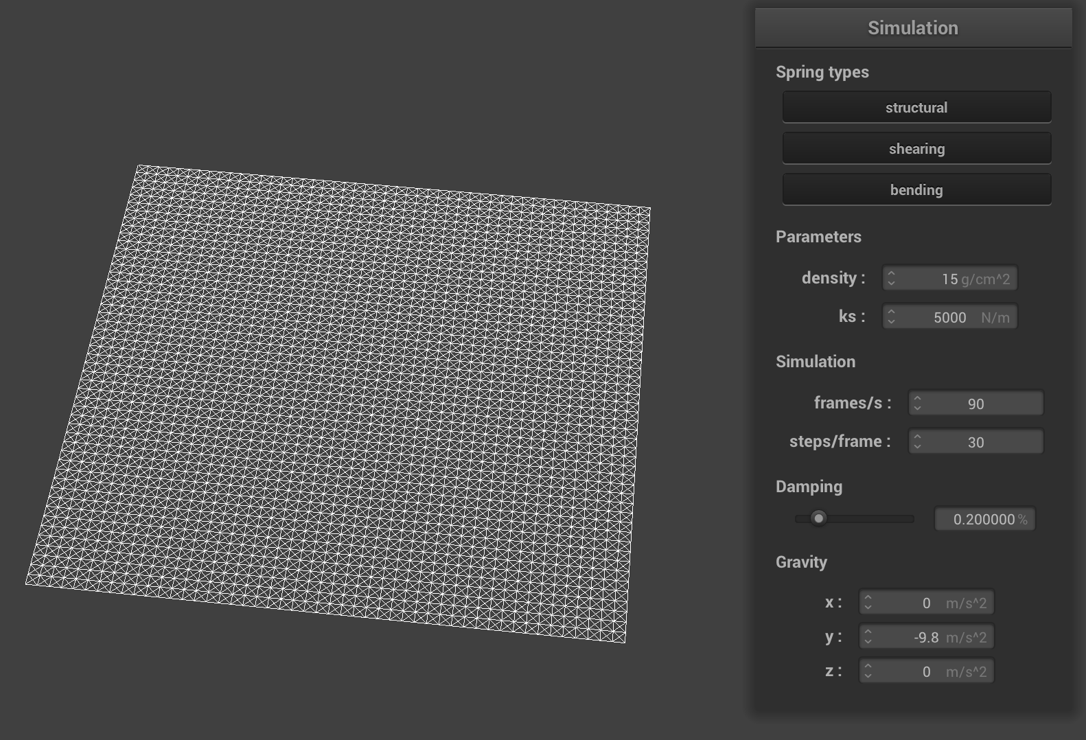 structural, shearing, and bending
|
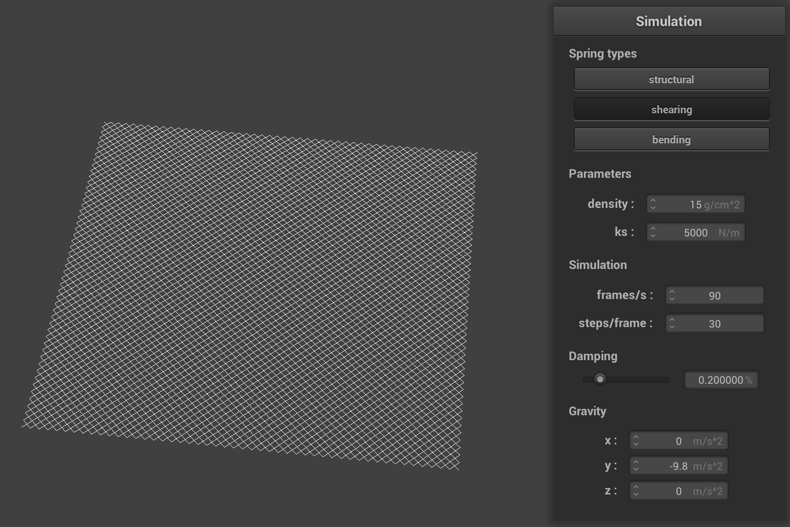 shear only
|
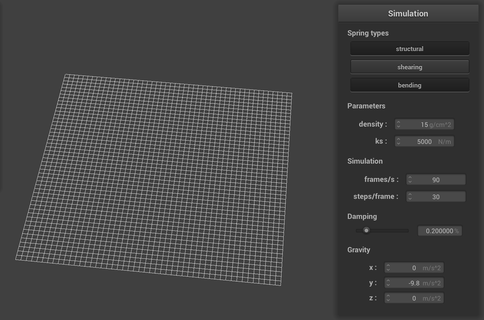 structural and bending
|
Part II: Simulation via Numerical Integration
The next part involved applying forces to point masses to simulate realistic movement. I calculated both external forces like gravity and spring correction forces. To get the total external force, I summed up all of the external accelerations and multiplied by the mass. For the correction forces, I used Hooke’s Law to compute the force applied to the point masses that connect the spring. I multiplied the spring constant by the magnitude of the distance between masses and subtracted the spring’s rest length. This is the force for one mass and the other has an equal (but opposite) force. Next, I used Verlet integration to calculate new point mass positions. To simulate damping, I multiplied a damping percentage by the difference between our new and last positions. I added the total acceleration and multiplied by the time-step squared. I add all of this to the current position, storing the position from the last time step as well. Fiinally , I made sure to constrain position updates by making sure that the spring’s new length is at most 10% greater than its rest length. I scaled with a correction vector and made sure that the vector direction was unchanged.
 density: 15 g/cm^2 & ks: 5000 N/m
|
 ks 9000
|
 ks 1000
|
Changing the spring constant ks creates visible changes in the cloth. When the constant is increased, the cloth springs up a little and it appears lighter in the simulation overall. When the constant is decreased, the cloth droops deeper and creates an effect of being much heavier.
 density 1
|
 density 100
|
I decreased the density to 1, which made the cloth super light. There were barely any folds and it looked almost paper-like. When increasing the density to 100, the cloth hangs lower and has much deeper folds, when comparing it to the default density of 15.
 damping 0.1
|
 damping 0.9
|
Turning down the damping causes more oscillation in the cloth. To slow down the oscillation, we increase the damping which acts opposite to the direction of motion.
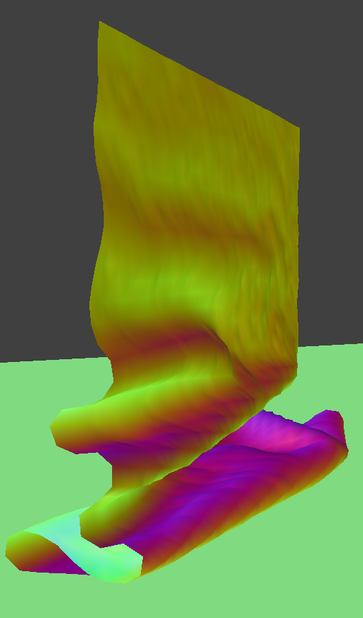
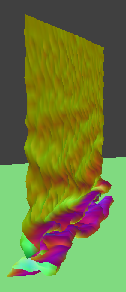
 pinned4 with density: 30 g/cm^2 & ks: 1000 N/m
|
Part III: Handling Collisions With Other Objects
I first handled collisions with spheres, which was a bit simpler for me than intersection with planes. I calculated where the point masses should have rested on the spheres surface by comparing the distance from the origin to the point mass’s position to the radius of the sphere. I computed a correction vector using the surface intersection tangent point and applied it to the last position of the point mass and scaled by friction. I updated the simulate method to test for intersection with all of the collision objects, as well. For plane intersection, if the point mass passes over the plane, I calculate a tangent point of where the mass should have rested. Using dot products of the mass’s current and last positions with the normal, I could determine whether that mass has passed through the plane or not. If so, I use the tangent point, a correction vector, and a small surface offset to adjust the mass’s last position, finally setting it to the current position.
With a larger ks value, the cloth has less weight and bounces back up towards the top of the sphere when changed mid-simulation. With a lower ks, the cloth begins to droop more.
 ks 500
|
 ks 5000
|
 ks 50000
|
 plane intersection
|
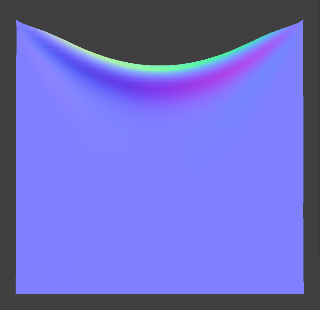
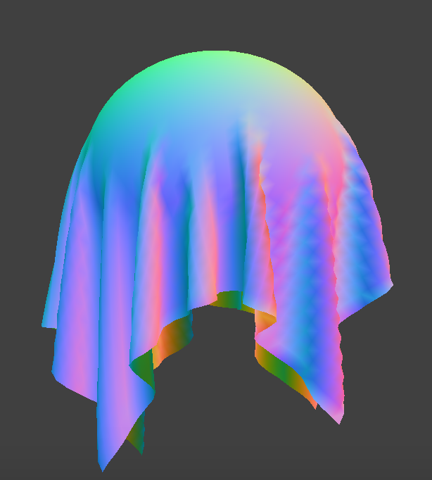
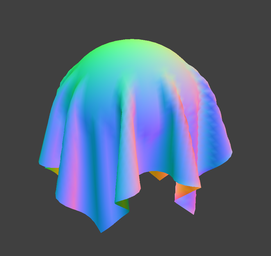
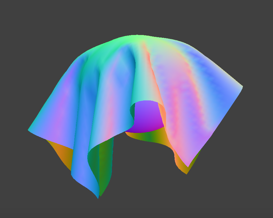
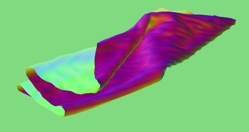
Part IV: Handling Self-Collisions
In order to keep the cloth from clipping though itself, I implemented a fix for self-collisions. Instead of looping through each pair of point masses, I used spatial hashing. Spatial hashing involves mapping a float to a vector of point masses. By creating a hash function that can uniquely map each point map position to a float, we can store points in boxes that represent specific 3D box volumes. For each point mass, we loop through the other masses that are most likely to collide with it. Thus, we can take all of the other masses in our 3D box (represented by a specific hash bucket) and compare them easily to our current mass. A small issue I had was forgetting to check if the hash bucket is not initially null. If so, I needed to populate it with a vector, since the current point mass would be the first member of that bucket.
 3 seconds in
|
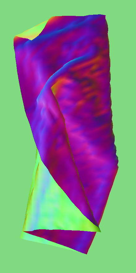
 about 9 seconds in
|
 resting state
|
 resting state top view
|
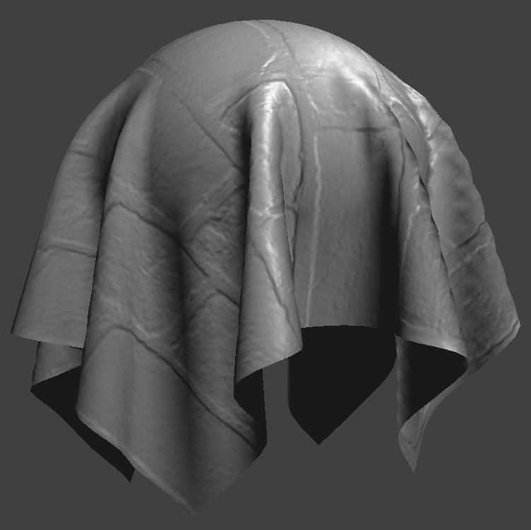
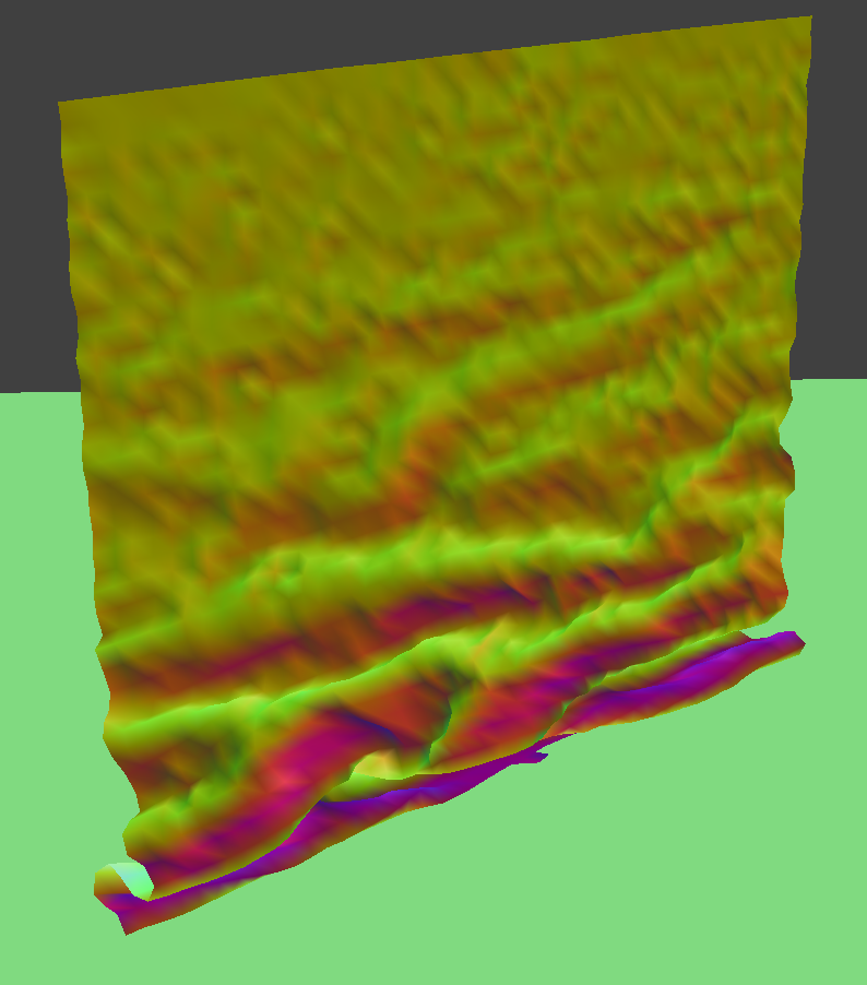
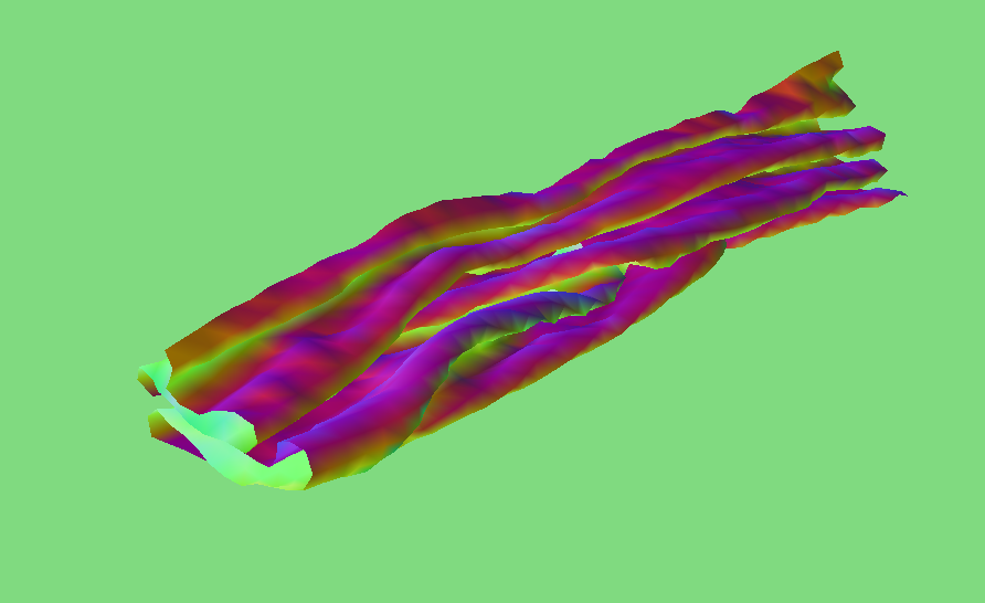
Below are images of the cloth with the density and ks values changed from the defaut values. When the ks is increased, there are larger folds with less wrinkles and the cloth appears more stiff. With a lower ks value, there are more wrinkles and the cloth is less stiff. Increasing the density created many more folds while decreasing density created wider folds with a more neat, less wrinkly resting state.
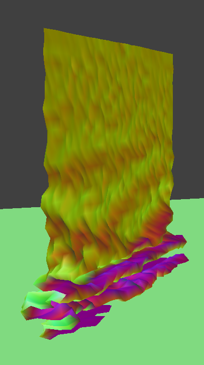 ks 2000
|
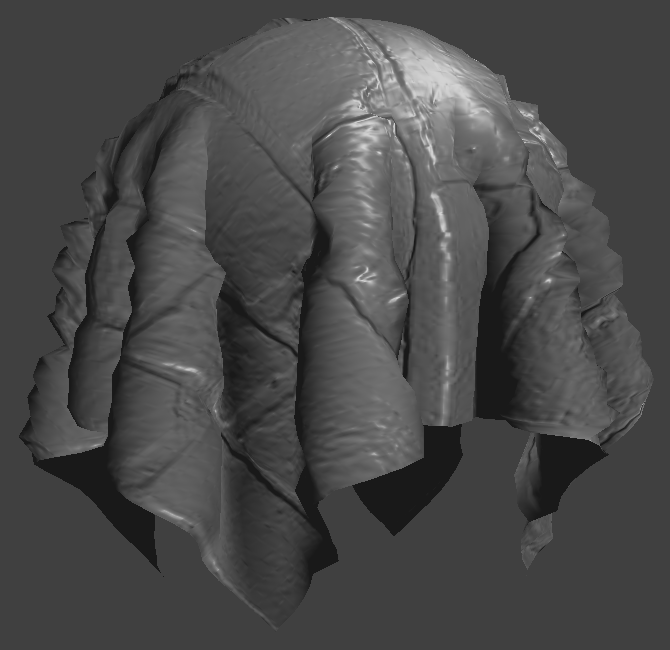
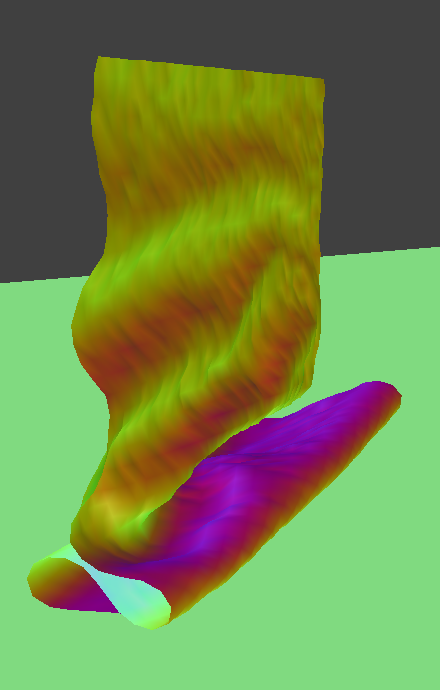 ks 50000
|
 density 5
|
 density 40
|
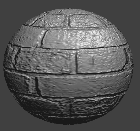
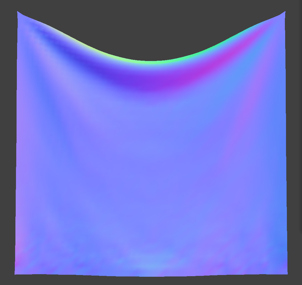
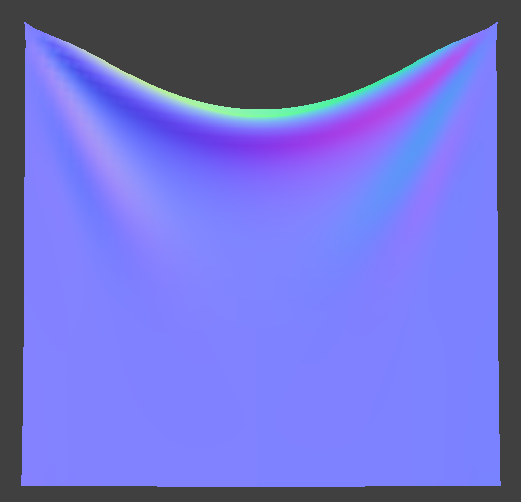
Part V: Shaders
In this section, I implemented some GLSL shaders, which run parallel on GPU, speeding up render time from the raytracing done in previous projects. GLSL is a language that has two basic shader types that take inputs and give back a 4-dimensional vector: vertex shaders and fragment shaders. Vertex shaders apply transforms to verticies while fragment shaders compute output colors.
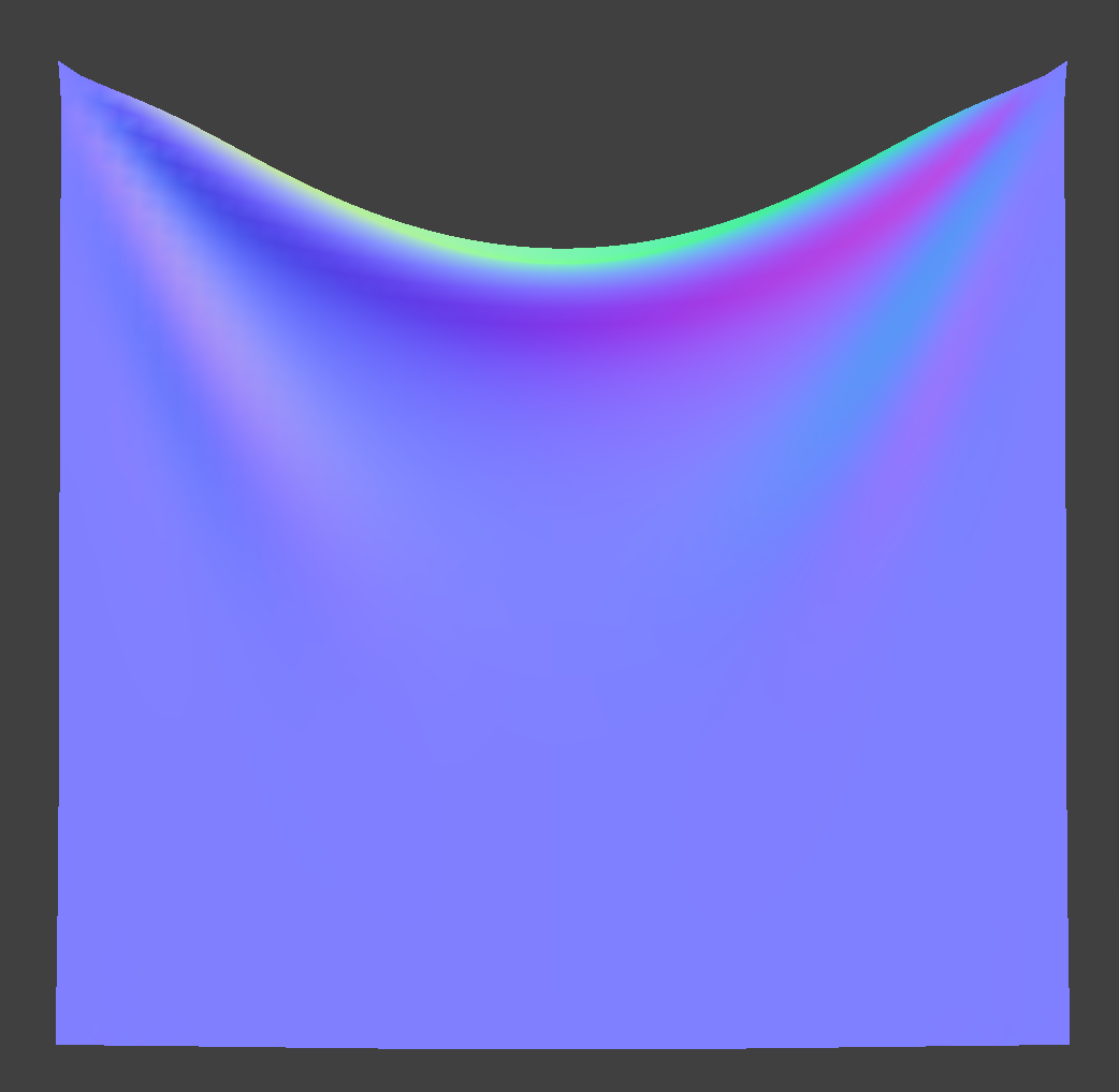
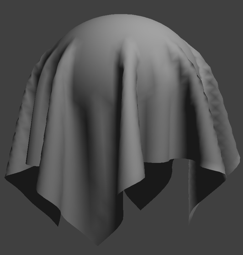
I first implemented diffuse shading, which uses the formula for diffuse lighting: Ld = kd(I/r^2)max(0, dot(n, l)). This was a fragment shader, so I wrote the final color to out_color.
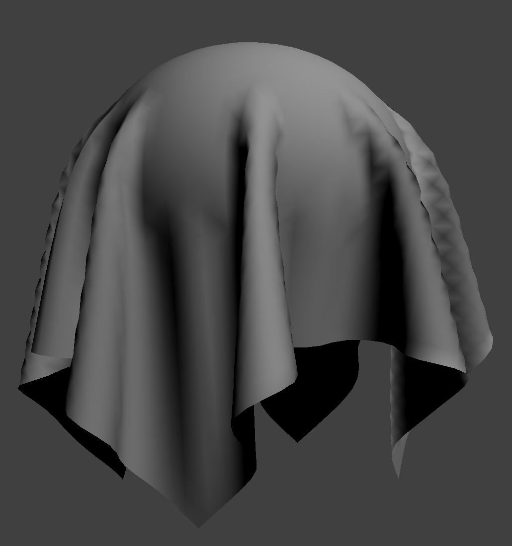 diffuse shader
|
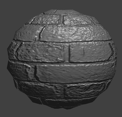
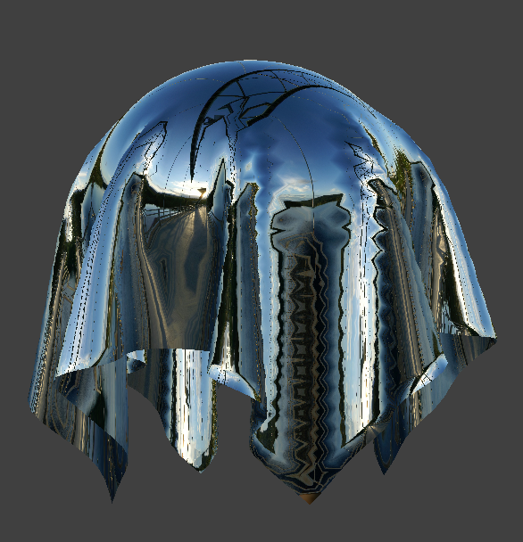
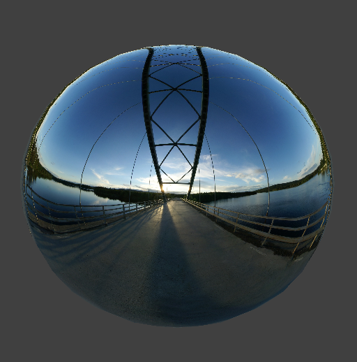
For Blinn-Phong shading, I built upon the diffuse shader to add ambient light and specular components and compute the output light. Below are the effects of isolating different components of the shader as well as the entire Blinn Phong model.
 ambient
|
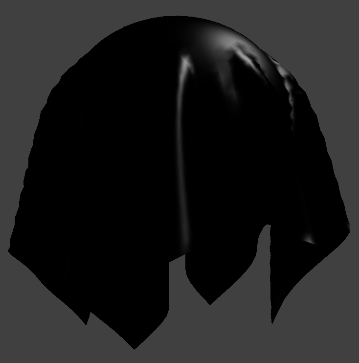 specular
|
 diffuse
|
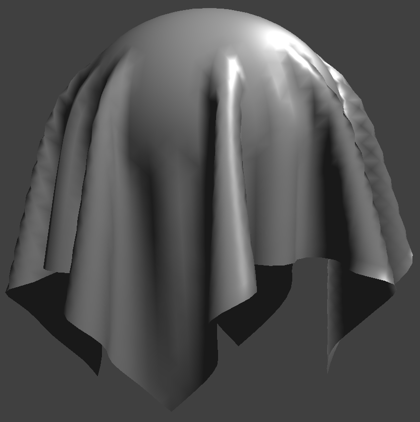 Blinn Phong
|
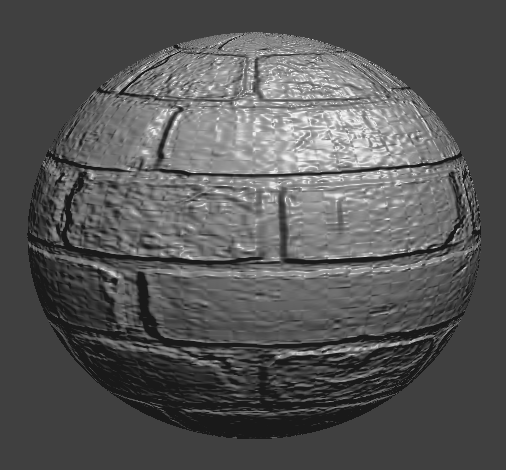
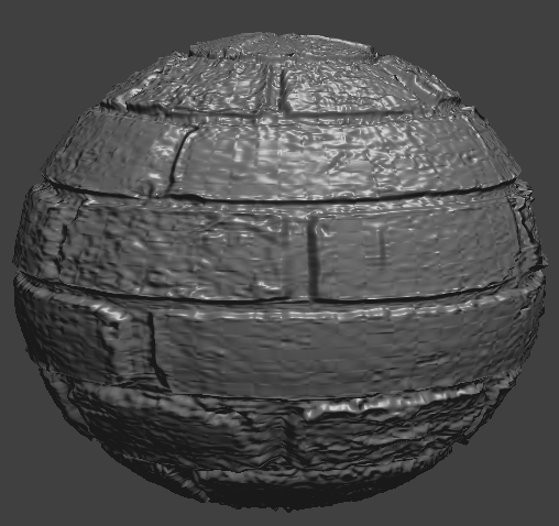
For texture mapping with GLSL, I sampled from a texture that I chose using the built-in texture(tex, uv) function.
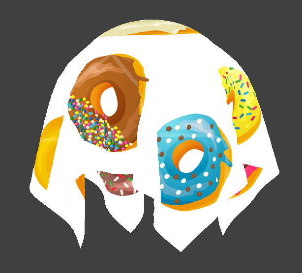 my donut texture!
|