Assignment 3-2: PathTracer

First, I implemented reflective and mirror materials. For the reflective surface, I used a reflective function which redirects the wo vector about the normal (0, 0, 1). I stored this in *wi and returned the reflectance divided by the cosine of the incoming vector. Since this is a perfect reflection, the function can just return the reflectance divided by the cosine of the vector with the normal. Glass was a bit more complicated and required the use of Snell’s law and equations. The eta value used in the calculations depended on whether the vector was “entering” or “exiting” the surface. In the refraction function, I determined whether total internal reflection occurred and if so we set the pdf to 1 and return the reflectance divided by the cosine of *wi. If not, reflection and refraction both occur, so we can compute Schilck’s reflection coefficient R to get a coin flip probability that tells us to either reflect or refract. Finally, I computed either the outgoing reflection/refraction, radiance, and its direction.

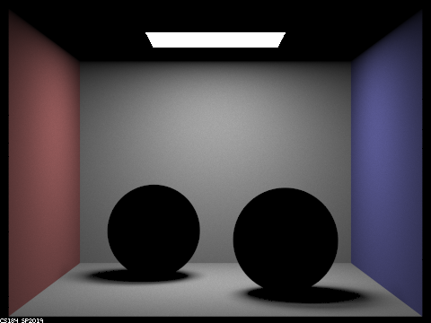
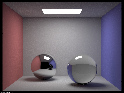
Below are images of the reflective and refractive materials with increasing max ray depths.

At depth 0 we just get the zero-bounce of the light source. Only materials directly illuminated by the light are visible, leaving the spheres black at depth 1.

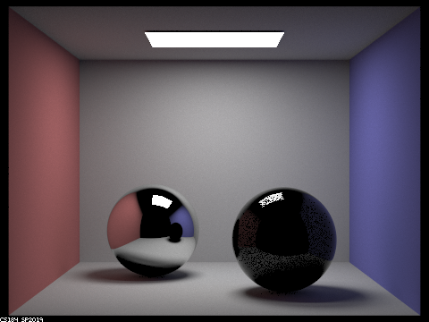
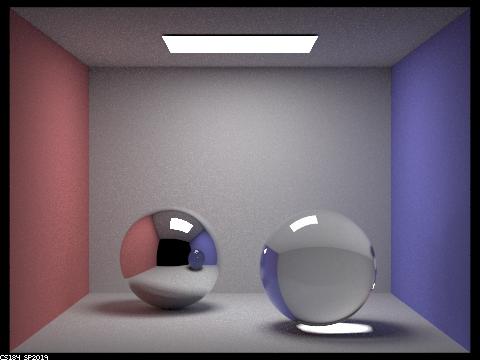
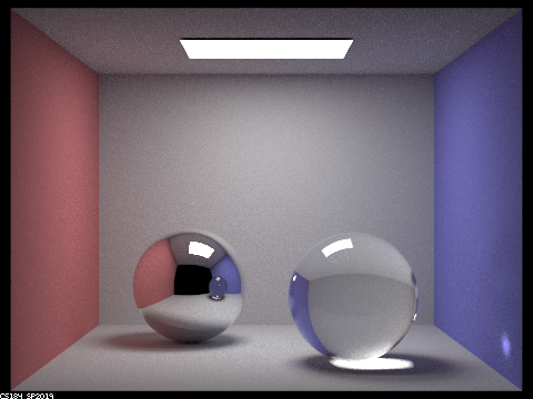
The mirror material is visible after 2 bounces, but we need one more bounce for the glass to get the effect of the light going through the material. At depth 3 we finally can see the glass material, but it’s shadow lacks a bright highlight. The glass also still appears dark in the mirror’s reflection.

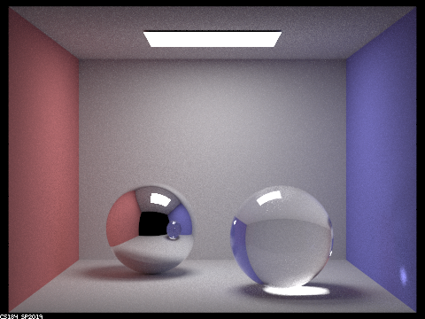
With depth of 4, we can see that highlight in the shadow from the glass refraction and the glass appears lighter in the mirror ball’s reflection. At depth 5, we can see a bounce of light appear on the purple wall. The jump from depth 5 to 100 isn’t that drastic, since there are no new refraction or reflection effects.

Part 2: Microfacet Material

The first step of implementing microfacet material was calculating the normal distribution function(NDF). Calling this function on the half vector h gives us the normals that are exactly along the vector, which can reflect wi-wo. The NDF uses the alpha value, or roughness of the material, which gives us a more glossy material when it is small and a more rough material when it is large. Next, I calculated the Fresnel term by calculating terms for each individual RGB value at fixed wavelengths. The last step was implementing BRDF importance sampling, in which I placed a higher priority on pdfs most similar to the D(h) call (NDF), ultimately creating less noise. Using the inversion method, I calculated the theta and phi values. I then calculated the pdf of sampling h solid angle and the final pdf of wi solid angle.

Below are renders at various alpha values. The alpha at .005 causes the material to be extremely smooth and shiny and it is slightly less smooth at .05. At .25 we start to see a larger difference and the material is more rough/diffuse. The material is very rough at .5 and we can notice the effects of the microfacet implementation the most here with a shiny, yet overall rough look.

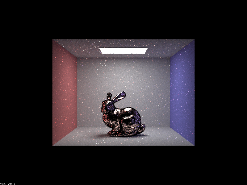
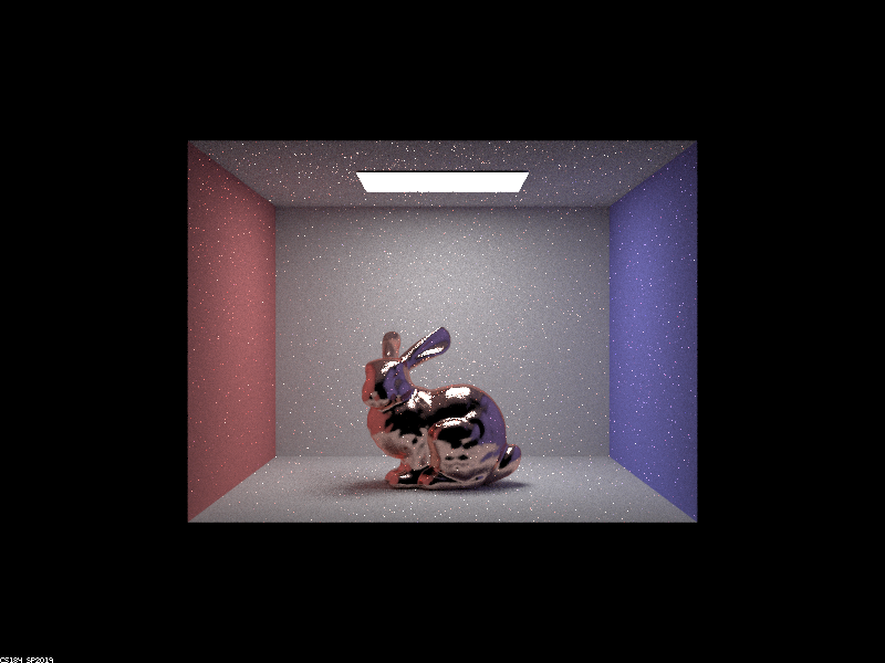
The cosine hemisphere sampling appears much more noisy than the importance sampling, especially in the lower parts of the bunny with the large highlight. The importance sampled render is overall a bit brighter and the copper material is more realistic.

I edited the eta and k values and made them equivalent to those of a platinum material.

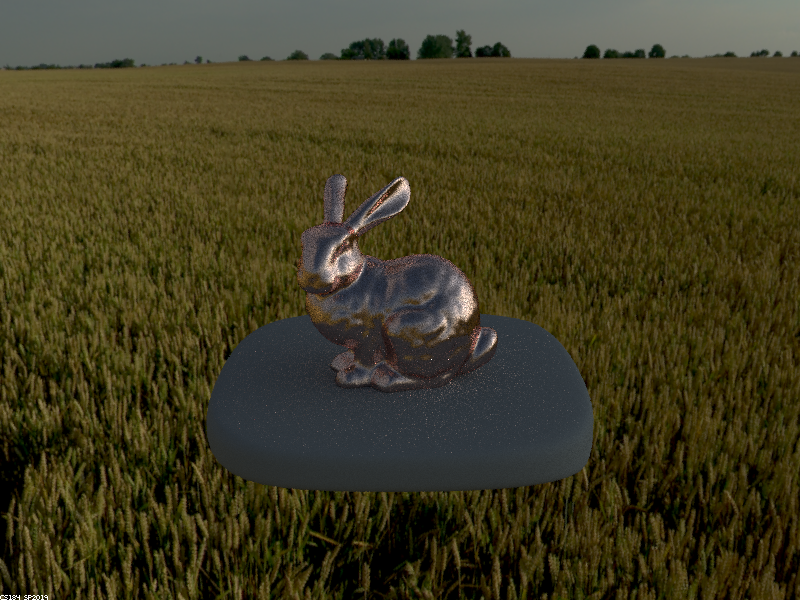
Part 3: Environment Light

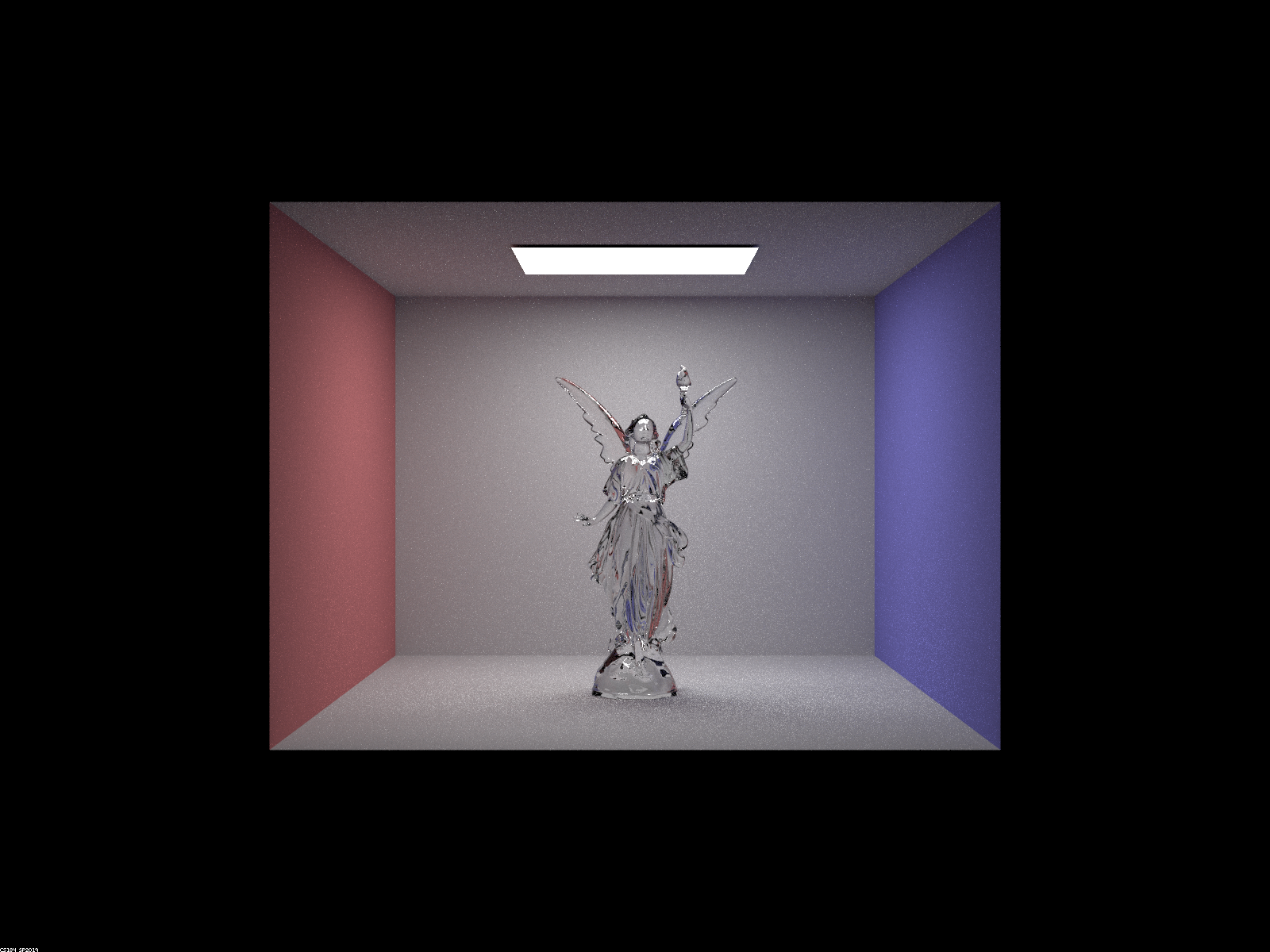
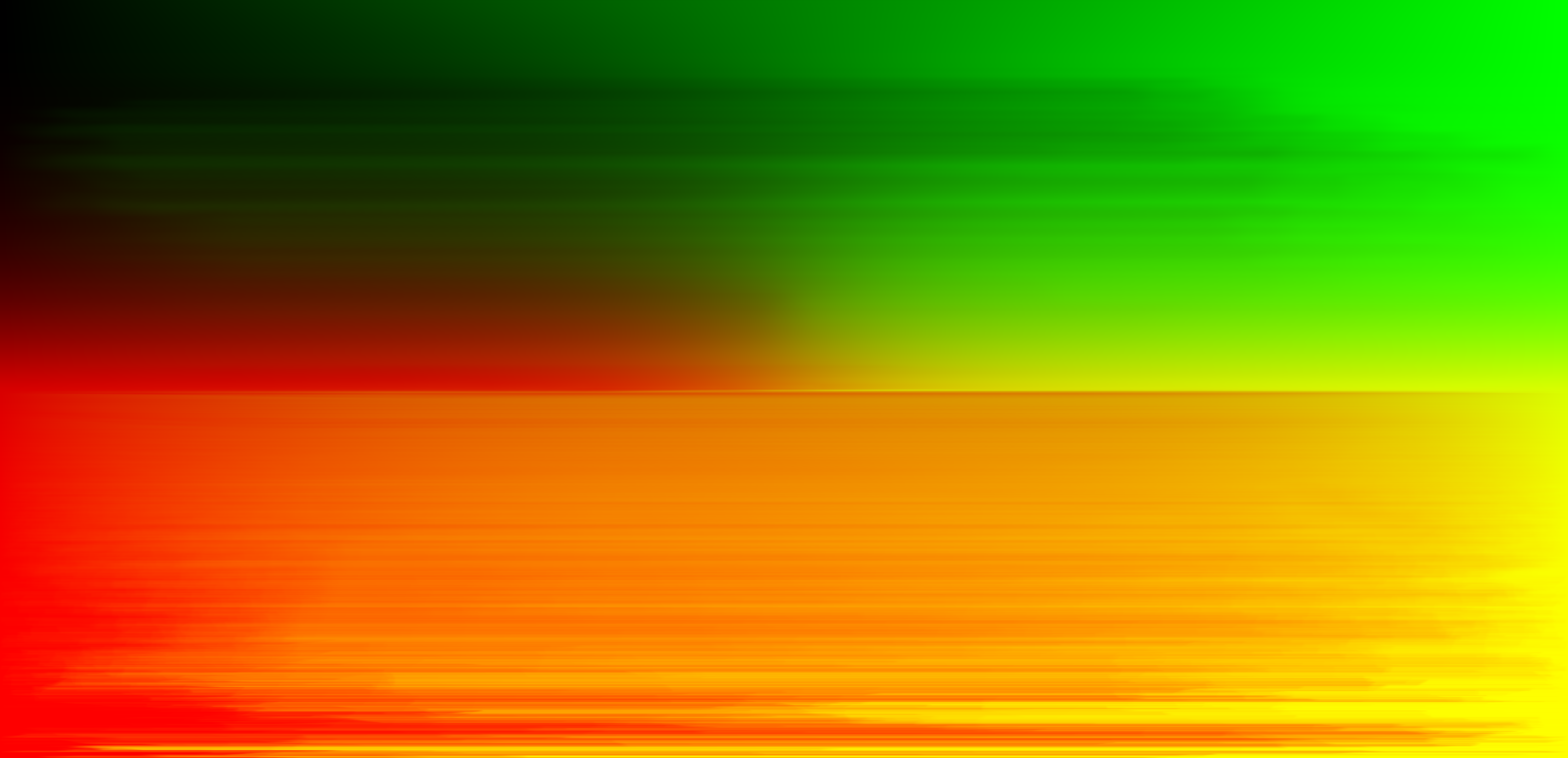
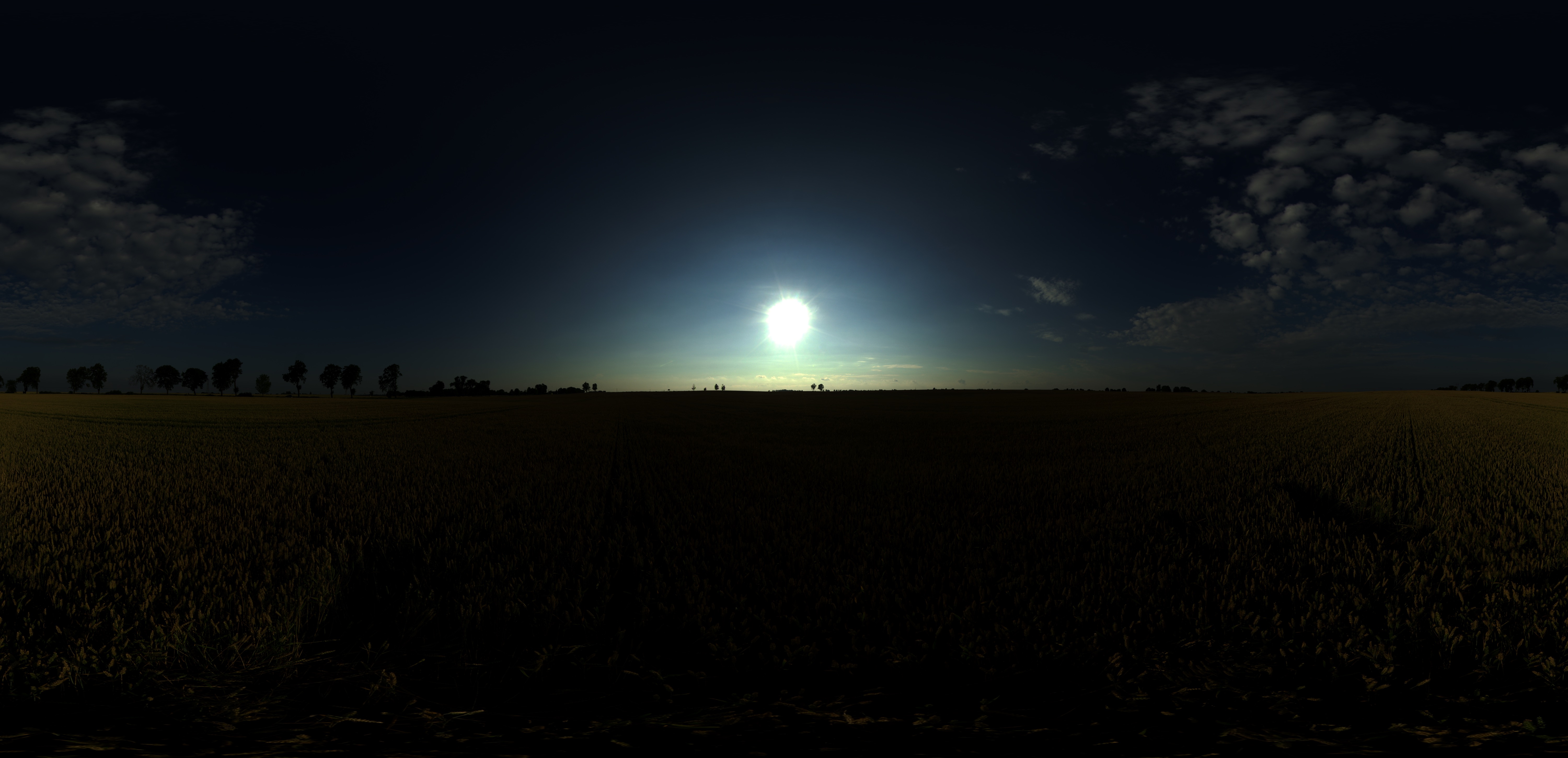
In this part, I implemented environment lighting. Environment lights supply radiance from all directions from an “infinite” distance to resemble realistic outdoor lighting. We implement environment lighting to get as close to realistic lighting as possible and we can define the intensity of light from different directions with a texture map like the one below.

The first part included the conversion of coordinates that were used to index into the environment map, placing the map in the back of the scene. The second part of this implementation, uniform sampling, included generating a random direction on the sphere with a 1/4pi uniform probability (pdf). I converted the direction to coordinates and found the radiance in the texture with bilinear interpolation. To decrease noise, I added importance sampling, which places a higher priority on samples where light is the brightest. Implementing importance sampling was trickier and more math-heavy, since it involved assigning a probability to each pixel in the map. I calculated the pdf for each index, since we want the information about relative radiance values at different points. I computed the marginal distribution p(y) next, retrieving its CDF given by:

F(j)=∑​j​′​​=0​j​​∑​i=0​w−1​​p(i,j​′​​)

Next, I calculated the conditional distributions and stored the values in the conds_y array. The debug image above verifies that the marginal and conditional distributions are correct. Finally, I updated sample_L to get a uniform sample, retrieve (x, y) values sampled from the pdf and convert them to a direction, calculate the pdf, and return the map value at (x, y).

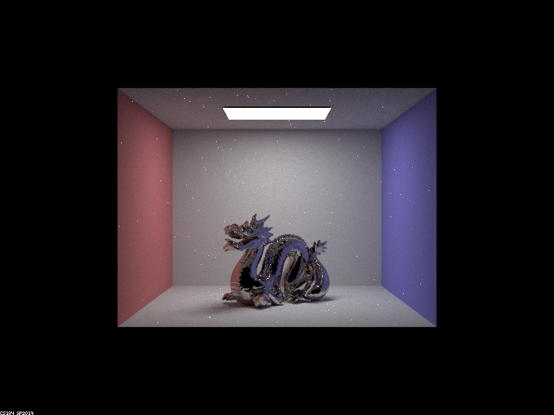
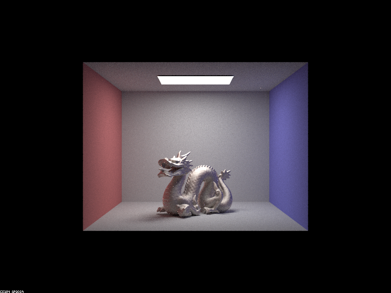
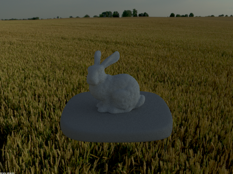
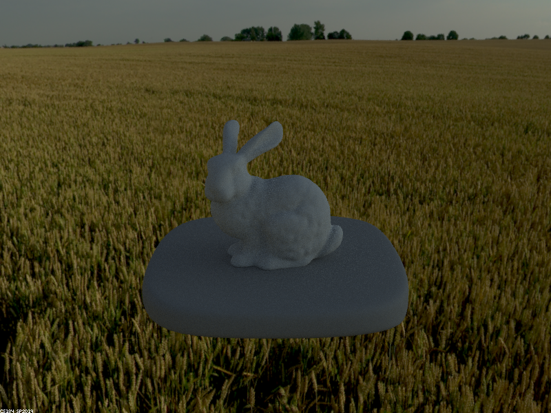
The noise levels in highlights and on the pedestal are decreased in the importance sampled render. The uniform sampled redner is overall a bit darker than the importance image.

Highlights appear brighter in the importance sampled render, since there is less noise. Like the previous unlit comparison, the importance image here is overall lighter, especially on the left side of the map. The copper material looks more realistic, as well.

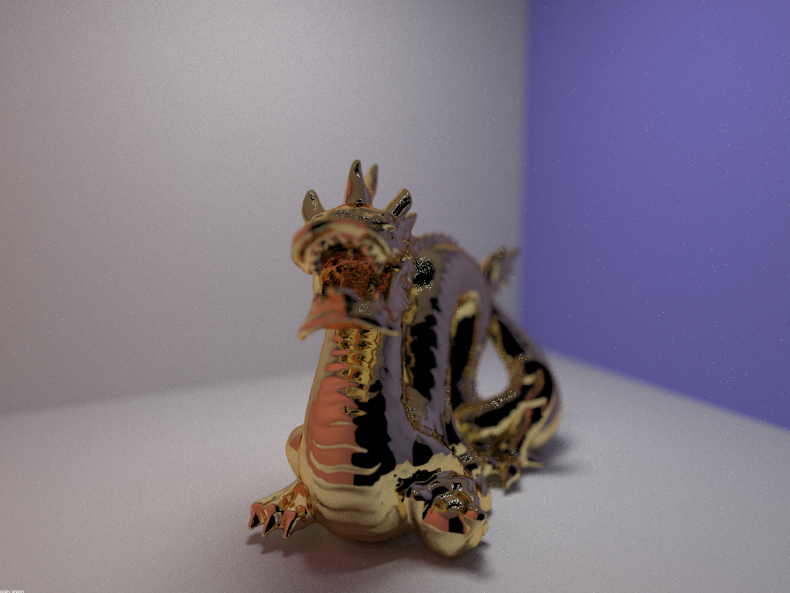
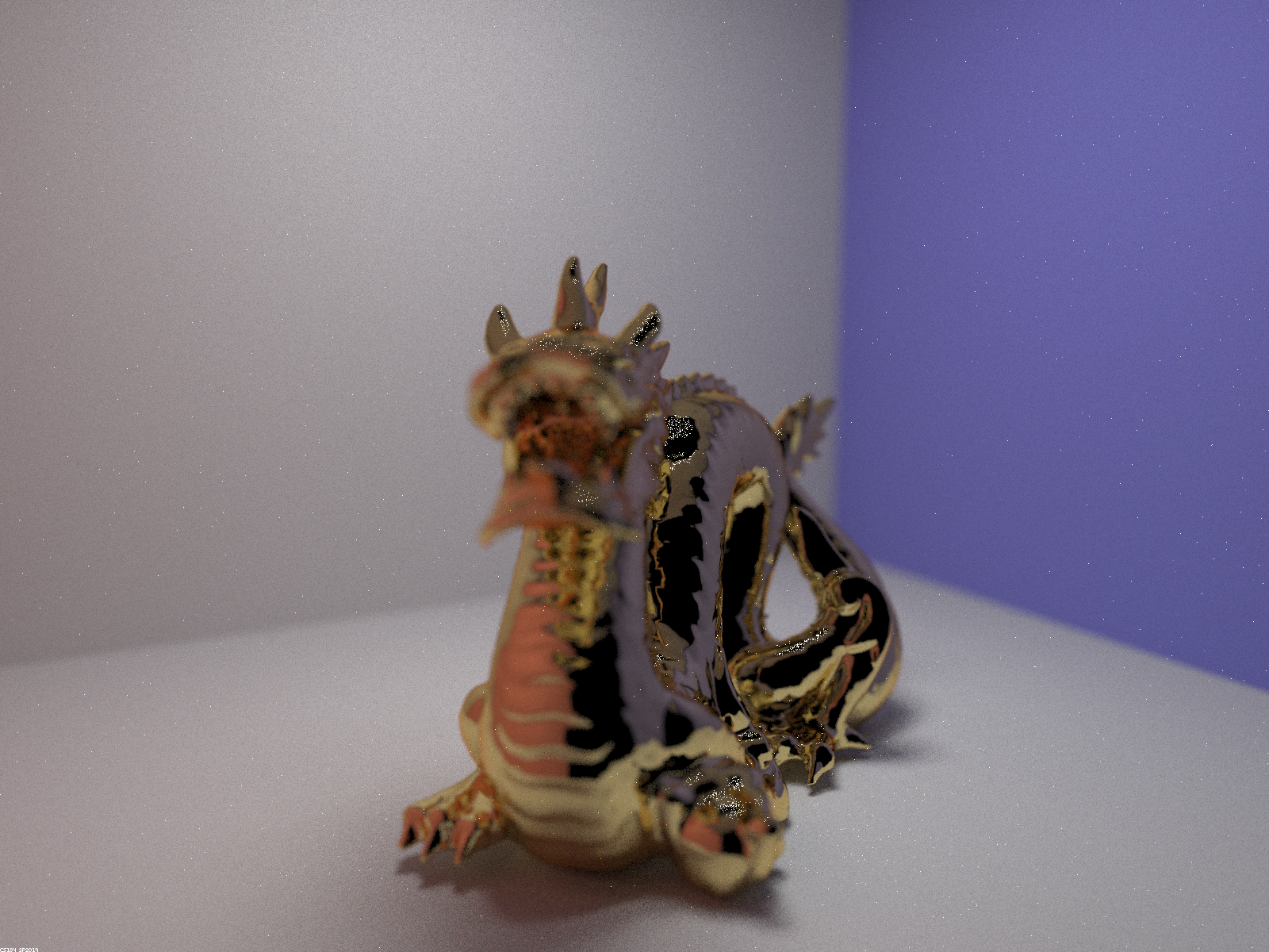
Part 4: Depth of Field

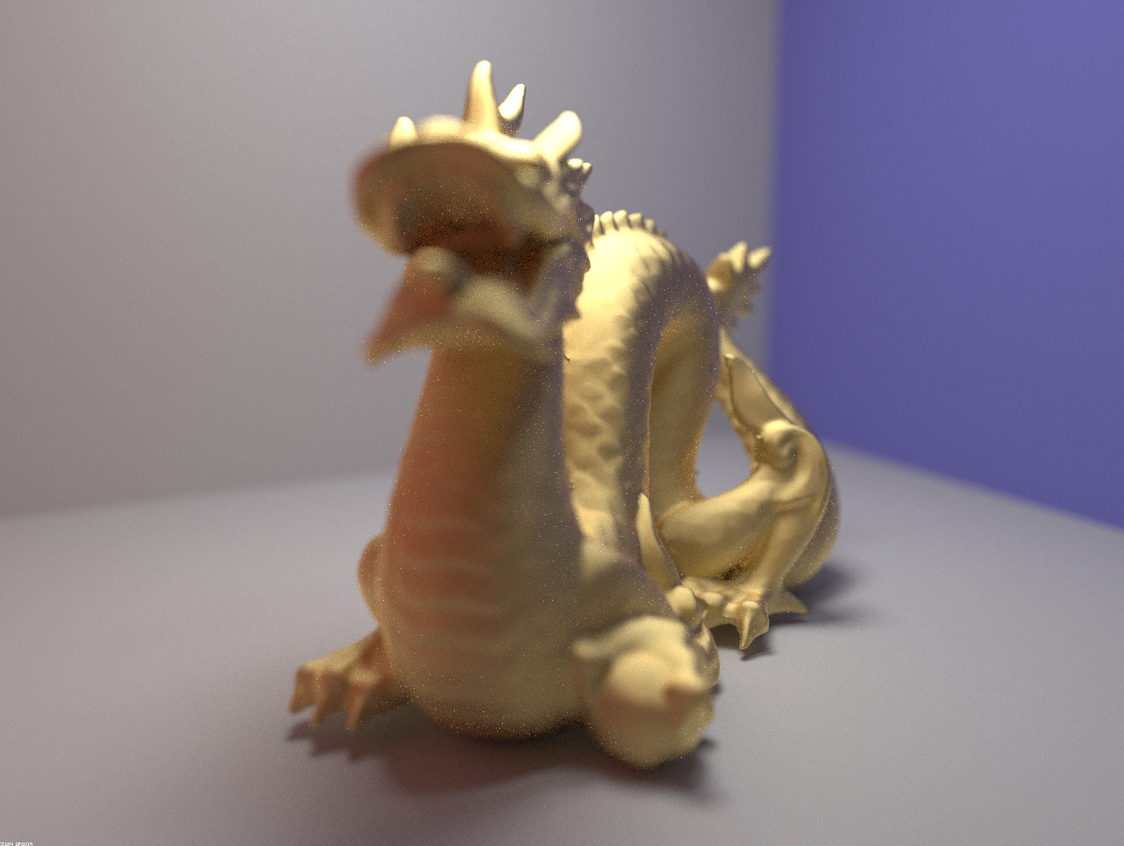
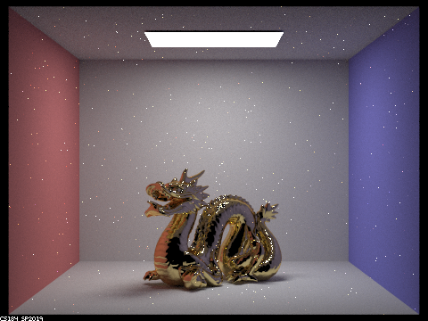
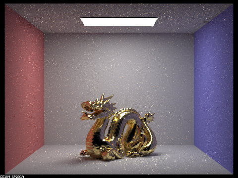
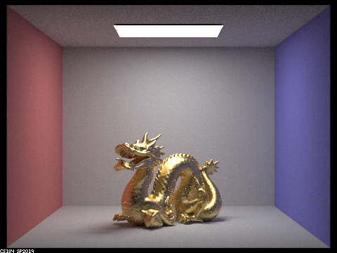
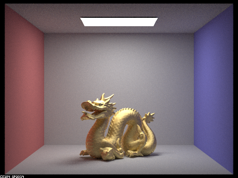
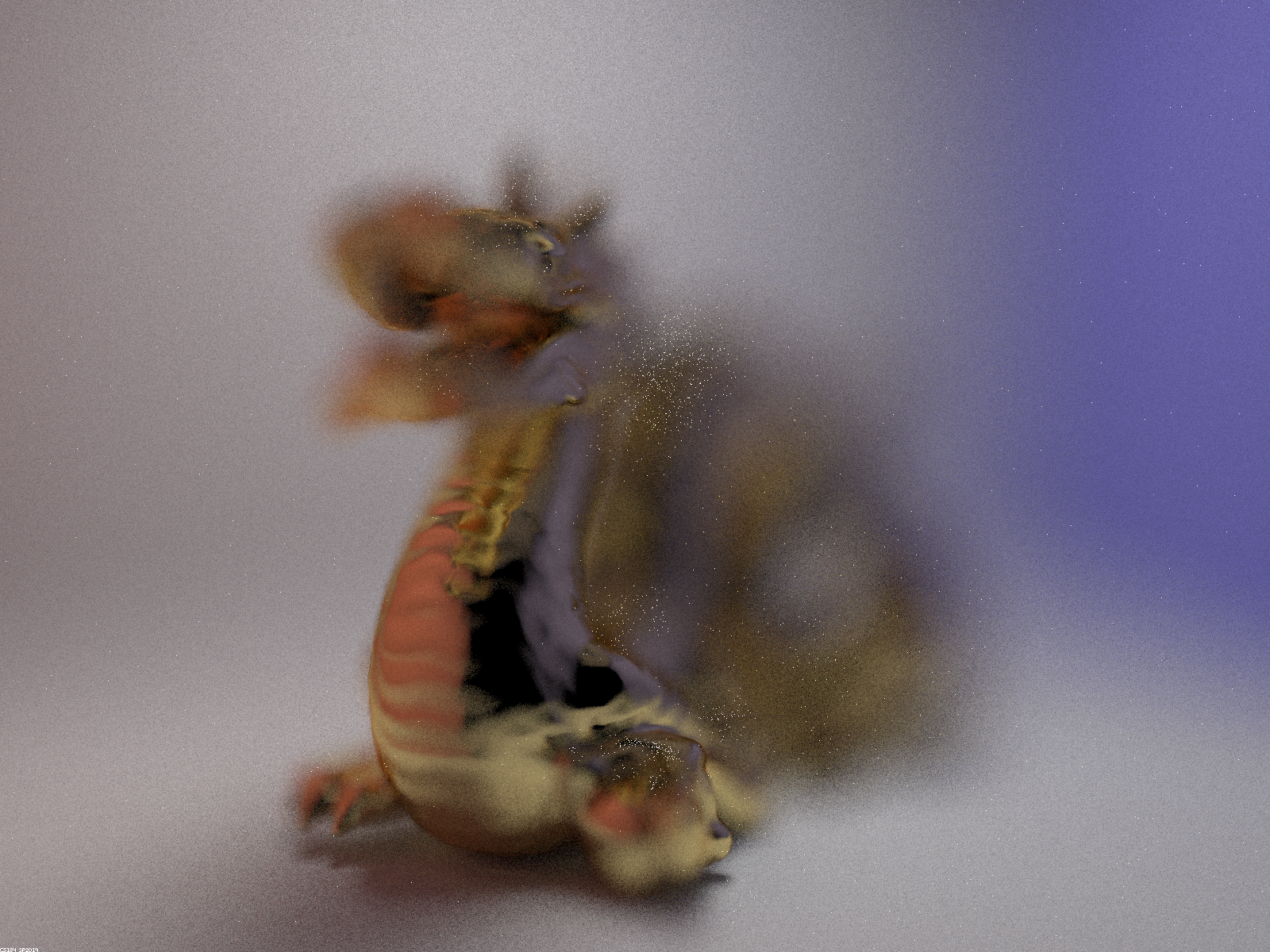
To render all of the previous images I was using the pinhole camera, which has everything in the scene in focus. In this part, I implemented a thin lens camera that allows only certain parts of the scene to be in focus based on focal distance and aperture. Only parts of the scene at the focal distance from the camera will be in focus. The sensor plane will be able to receive radiance from many locations, not only from (0, 0, 0). First, I calculated the ray direction and uniformly sampled the thin lens disk using uniformly distributed parameters rndR and rndTheta. I calculated a pFocus value by multiplying the focal distance by the ray’s direction and subtracted that value from the center of the lens. Next, I calculated a ray whose origin is the uniform sample and whose direction is towards pFocus. Finally, I converted coordinates to world space and set the nClip and fClip values. Below are images rendered at various focal distances and aperture values.

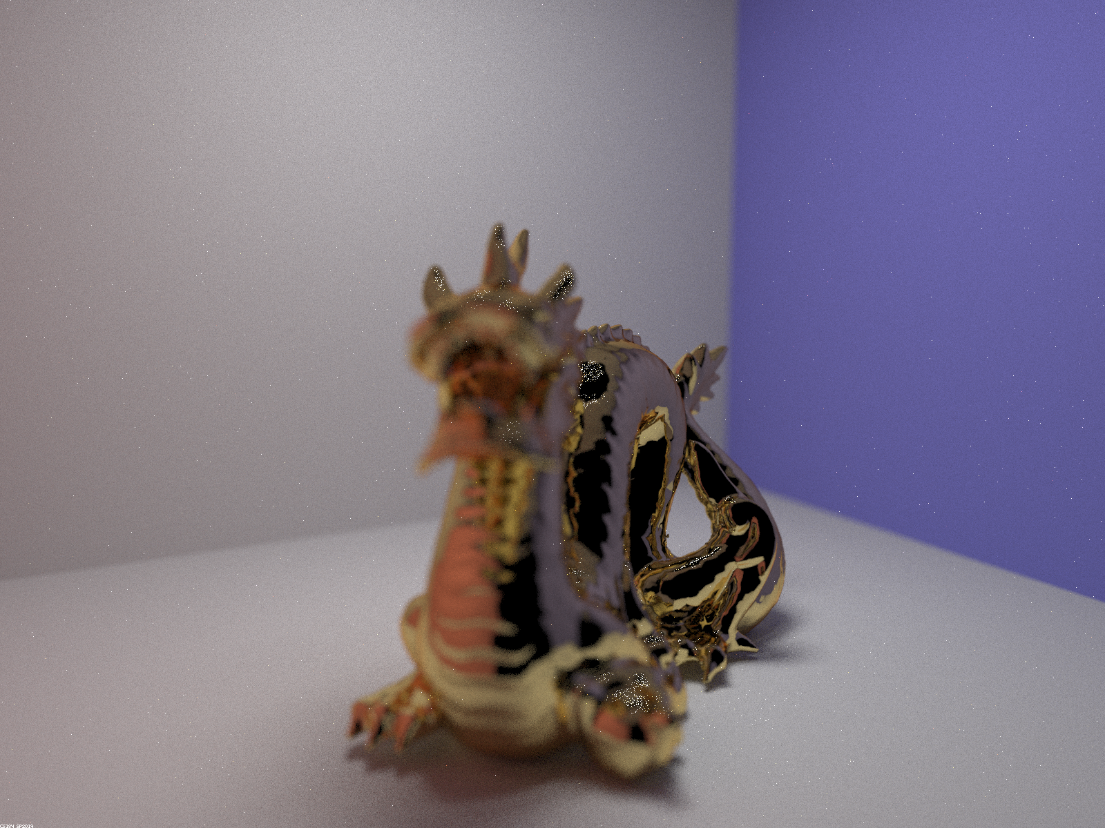
From this angle, as the focal distance gets larger, the focus shifts to points further back on the dragon.

Increasing aperture causes the out-of-focus parts of the image to become even more blurred and fuzzy.